The goal of the package is to create a vector representation of acceleration bursts in R. Acceleration bursts are a frequently collected by animal tracking devices and consist of measurements of the acceleration in one till three axis. These measurements are recorded with a fixed frequency for a few seconds. These burst are frequently considered one “instantaneous” sample of the activity or behavior of an animal.
By creating a vector representation it becomes more easy to manipulate these bursts and for example add them to a data frame.
Creating a burst
To create a acceleration vector a list of acceleration measurements are combined with the measurement frequency. Each element of the list is a matrix with the columns being the axis the acceleration is measured in and the rows being the repeated measurements.
x <- acc(
  bursts = list(cbind(
    x = sin(1:30 / 10),
    y = cos(1:30 / 10),
    z = 1:30 / 10
  )),
  frequency = units::as_units(40, "Hz")
)
x
#> <acceleration[1]>
#> [1] (0.67 0.01 1.55)
#> # frequency: 40 [Hz]
When printed it reports the average acceleration for each axis of each burst and the measurement frequency. Multiple bursts can be combined with diverse properties can be combined.
y <- acc(
  bursts = list(
    cbind(x = sin(1:20 / 10), y = cos(1:20 / 10)),
    cbind(x = sin(1:20 / 10 + 2), y = cos(1:20 / 10 + 3))
  ),
  frequency = units::as_units(30, "Hz")
)
y
#> <acceleration[2]>
#> [1] (0.73 0.42)  (0.08 -0.52)
#> # frequency: 30 [Hz]
c(x, y)
#> <acceleration[3]>
#> [1] (0.67 0.01 1.55) (0.73 0.42)      (0.08 -0.52)
#> # frequency: 30 [Hz] - 40 [Hz]
Loading data
Naturally most of the time data won’t be generated directly in R but
rather loaded from local files or databases like movebank. For data from
movebank some quick conversion options have been build. These take
move2 objects as an input. For now conversion functions for
data from eobs and ornitella tags exists.
Here is an example for eobs tags. When the as_acc
function is applied to a move2 it attempts to detect the
columns representing the acceleration data.
require(dplyr, quietly = TRUE)
#>
#> Attaching package: 'dplyr'
#> The following objects are masked from 'package:stats':
#>
#> filter, lag
#> The following objects are masked from 'package:base':
#>
#> intersect, setdiff, setequal, union
require(move2, quietly = TRUE)
kinkajous_data <- movebank_download_study("Kinkajous on Pipeline Road Panama",
sensor_type_id = c("acceleration", "gps"), "license-md5" = "6e1743b4b2a919df0f3b4167c94786d9"
)
#> ℹ In total 1866 records were omitted as they were not deployed (the
#> `deployment_id` was `NA`).
kinkajous_data <- kinkajous_data %>%
mutate(acceleration = as_acc(.)) %>%
select(acceleration)
tail(kinkajous_data)
#> A <move2> with `track_id_column` "individual_local_identifier" and
#> `time_column` "timestamp"
#> Containing 1 track lasting 5.02 mins in a
#> Simple feature collection with 6 features and 3 fields (with 6 geometries empty)
#> Geometry type: POINT
#> Dimension: XY
#> Bounding box: xmin: NA ymin: NA xmax: NA ymax: NA
#> Geodetic CRS: WGS 84
#> # A tibble: 6 × 4
#> acceleration geometry timestamp
#> * <acc> <POINT [°]> <dttm>
#> 1 (2228.46 1869.85 2658.23) EMPTY 2010-01-22 17:58:00
#> 2 (2222.88 1871.77 2662.77) EMPTY 2010-01-22 17:59:00
#> 3 (2224.23 1865.04 2663.31) EMPTY 2010-01-22 18:00:00
#> 4 (2220.88 1864.19 2667.31) EMPTY 2010-01-22 18:01:00
#> 5 (2229.73 1862.54 2660.12) EMPTY 2010-01-22 18:02:00
#> 6 (2223.92 1870.85 2663.42) EMPTY 2010-01-22 18:03:01
#> # ℹ 1 more variable: individual_local_identifier <fct>
#> Track features:
#> # A tibble: 1 × 51
#> deployment_id tag_id individual_id animal_life_stage animal_reproductive_co…¹
#> <int64> <int64> <int64> <fct> <fct>
#> 1 2923527 2923517 2923505 adult lactating
#> # ℹ abbreviated name: ¹animal_reproductive_condition
#> # ℹ 46 more variables: attachment_type <fct>, deploy_on_timestamp <dttm>,
#> # duty_cycle <chr>, deployment_local_identifier <fct>,
#> # manipulation_type <fct>, tag_readout_method <fct>, sensor_type_ids <chr>,
#> # capture_location <POINT [°]>, deploy_on_location <POINT [°]>,
#> # deploy_off_location <POINT [°]>, individual_comments <chr>,
#> # individual_local_identifier <fct>, sex <fct>, taxon_canonical_name <fct>, …The same can be done with ornitella data.
d <- as.Date("2021-3-3")

lbbg_data <- movebank_download_study("LBBG_ZEEBRUGGE - Lesser black-backed gulls ",
  sensor_type_id = c("gps", "acceleration"),
  timestamp_start = as.POSIXct(d),
  timestamp_end = as.POSIXct(d + 1)
)
lbbg_data <- lbbg_data %>%
  mutate(acceleration = as_acc(.)) %>%
  filter(!is.na(acceleration) | sensor_type_id==653) %>%
  select(acceleration)
lbbg_data
#> A <move2> with `track_id_column` "individual_local_identifier" and
#> `time_column` "timestamp"
#> Containing 5 tracks lasting on average 23.3 hours in a
#> Simple feature collection with 378 features and 3 fields (with 59 geometries empty)
#> Geometry type: POINT
#> Dimension:     XY
#> Bounding box:  xmin: -6.418534 ymin: 35.70378 xmax: 2.975934 ymax: 50.48241
#> Geodetic CRS:  WGS 84
#> # A tibble: 378 × 4
#>    acceleration             geometry timestamp
#>           <acc>          <POINT [°]> <dttm>
#>  1           NA (0.9766757 49.94388) 2021-03-03 00:46:30
#>  2           NA  (1.216243 50.01877) 2021-03-03 01:46:31
#>  3           NA  (1.275341 50.04811) 2021-03-03 02:46:41
#>  4           NA  (1.273401 50.04827) 2021-03-03 03:07:07
#>  5           NA  (1.270243 50.04776) 2021-03-03 03:27:18
#>  6           NA  (1.265624 50.04643) 2021-03-03 03:47:19
#>  7           NA  (1.259936 50.04491) 2021-03-03 04:07:20
#>  8           NA  (1.253495 50.04293) 2021-03-03 04:27:36
#>  9           NA  (1.246066 50.04075) 2021-03-03 04:47:34
#> 10           NA  (1.237192 50.03854) 2021-03-03 05:07:33
#> # ℹ 368 more rows
#> # ℹ 1 more variable: individual_local_identifier <fct>
#> Track features:
#> # A tibble: 5 × 61
#>   deployment_id     tag_id individual_id alt_project_id animal_life_stage
#>         <int64>    <int64>       <int64> <fct>          <fct>
#> 1    1790632438  985147358     985147048 LBBG_ZEEBRUGGE adult
#> 2    1790632586  985147353     985147183 LBBG_ZEEBRUGGE adult
#> 3    1790632519  985147368     985147052 LBBG_ZEEBRUGGE adult
#> 4    1790632560  985147375     985147076 LBBG_ZEEBRUGGE adult
#> 5    1790632534 1218541489    1218541458 LBBG_ZEEBRUGGE adult
#> # ℹ 56 more variables: animal_mass [g], attachment_type <fct>,
#> #   deployment_comments <chr>, deploy_off_timestamp <dttm>,
#> #   deploy_on_timestamp <dttm>, deployment_end_type <fct>,
#> #   deployment_local_identifier <fct>, location_accuracy_comments <chr>,
#> #   manipulation_type <fct>, study_site <chr>, tag_firmware <fct>,
#> #   tag_readout_method <fct>, sensor_type_ids <chr>,
#> #   capture_location <POINT [°]>, deploy_on_location <POINT [°]>, …
mt_stack(lbbg_data, kinkajous_data)
#> A <move2> with `track_id_column` "individual_local_identifier" and
#> `time_column` "timestamp"
#> Containing 7 tracks lasting on average 149266 secs in a
#> Simple feature collection with 11247 features and 3 fields (with 10445 geometries empty)
#> Geometry type: POINT
#> Dimension:     XY
#> Bounding box:  xmin: -79.74329 ymin: 9.136739 xmax: 2.975934 ymax: 50.48241
#> Geodetic CRS:  WGS 84
#> # A tibble: 11,247 × 4
#>    acceleration             geometry timestamp
#>  *        <acc>          <POINT [°]> <dttm>
#>  1           NA (0.9766757 49.94388) 2021-03-03 00:46:30
#>  2           NA  (1.216243 50.01877) 2021-03-03 01:46:31
#>  3           NA  (1.275341 50.04811) 2021-03-03 02:46:41
#>  4           NA  (1.273401 50.04827) 2021-03-03 03:07:07
#>  5           NA  (1.270243 50.04776) 2021-03-03 03:27:18
#>  6           NA  (1.265624 50.04643) 2021-03-03 03:47:19
#>  7           NA  (1.259936 50.04491) 2021-03-03 04:07:20
#>  8           NA  (1.253495 50.04293) 2021-03-03 04:27:36
#>  9           NA  (1.246066 50.04075) 2021-03-03 04:47:34
#> 10           NA  (1.237192 50.03854) 2021-03-03 05:07:33
#> # ℹ 11,237 more rows
#> # ℹ 1 more variable: individual_local_identifier <fct>
#> Track features:
#> # A tibble: 7 × 63
#>   deployment_id     tag_id individual_id alt_project_id animal_life_stage
#>         <int64>    <int64>       <int64> <fct>          <fct>
#> 1    1790632438  985147358     985147048 LBBG_ZEEBRUGGE adult
#> 2    1790632586  985147353     985147183 LBBG_ZEEBRUGGE adult
#> 3    1790632519  985147368     985147052 LBBG_ZEEBRUGGE adult
#> 4    1790632560  985147375     985147076 LBBG_ZEEBRUGGE adult
#> 5    1790632534 1218541489    1218541458 LBBG_ZEEBRUGGE adult
#> 6       2923528    2923516       2923504 NA             adult
#> 7       2923527    2923517       2923505 NA             adult
#> # ℹ 58 more variables: animal_mass [g], attachment_type <fct>,
#> #   deployment_comments <chr>, deploy_off_timestamp <dttm>,
#> #   deploy_on_timestamp <dttm>, deployment_end_type <fct>,
#> #   deployment_local_identifier <fct>, location_accuracy_comments <chr>,
#> #   manipulation_type <fct>, study_site <chr>, tag_firmware <fct>,
#> #   tag_readout_method <fct>, sensor_type_ids <chr>,
#> # capture_location <POINT [°]>, deploy_on_location <POINT [°]>, …Plotting
With the plot_time function it is possible to explor the
acceleration bursts. In this plot you can zoom using your mouse.
Alternatively you can plot one burst directly, in this case showing the clear wing beats on the z axis.
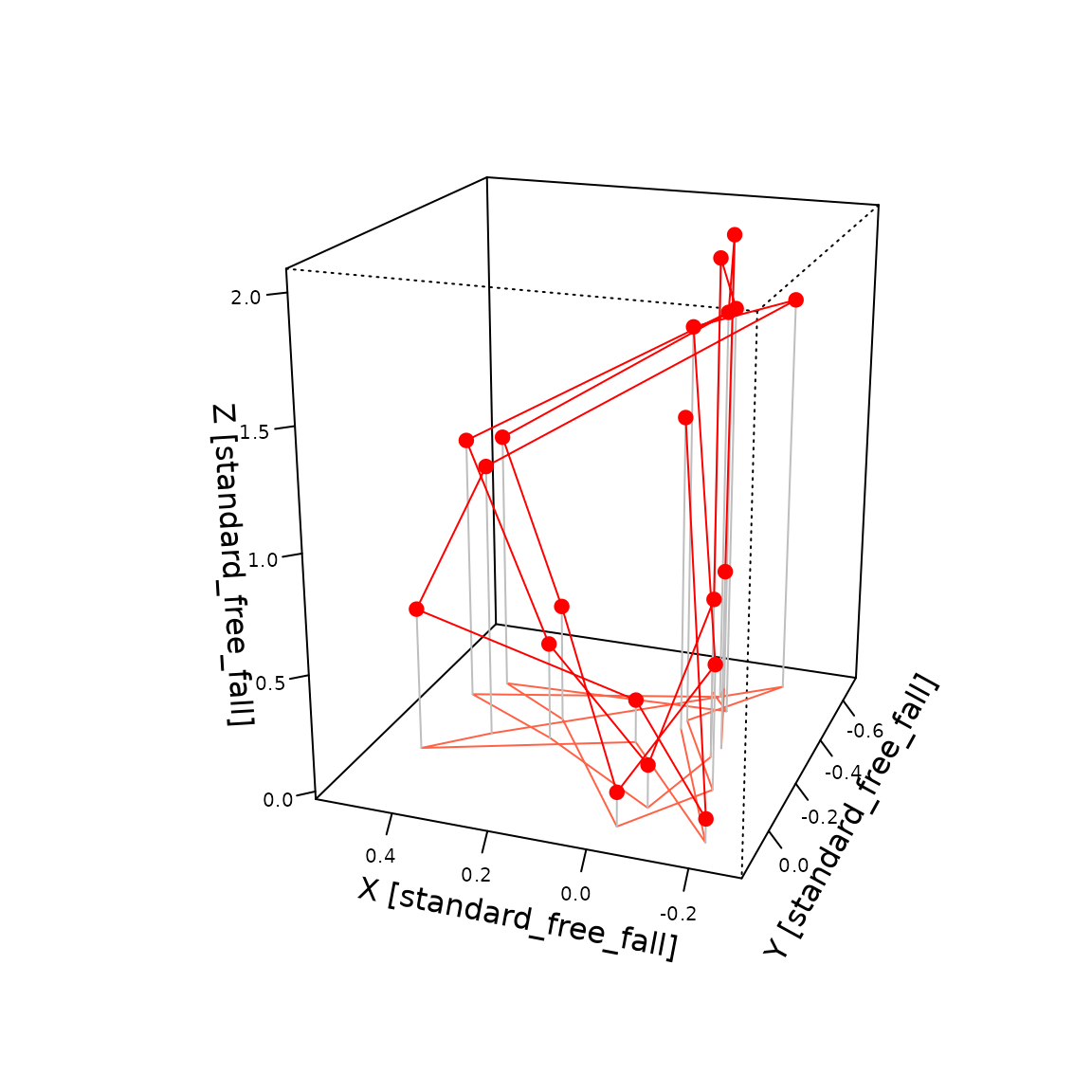
We can also visualize one burst in three dimensions showing the cyclic patterns in the acceleration.
bb<-vctrs::field(lbbg_data$acceleration[340],"bursts")[[1]]
b<-units::drop_units(bb)
e<-0.1
persp(z=matrix(min(b[,'tilt_z'])-e, ncol=2, nrow=2),
      x=range(b[,'tilt_x']),
      y=range(b[,'tilt_y']),
      xlim=range(b[,'tilt_x'])+c(-e,e),
      ylim=range(b[,'tilt_y'])+c(-e,e),
      zlim=range(b[,'tilt_z'])+c(-e,e),
      border=NA,
      xlab=paste0("X [",as.character(units(bb)),']'),
      ticktype = "detailed", cex.axis = 0.65,
      ylab=paste0("Y [",as.character(units(bb)),']'),
      zlab=paste0("Z [",as.character(units(bb)),']'),
      theta = -160, phi = 20, expand = 0.5, col = "white", scale=F)->p
# Draw line on bottom of plot
lines(trans3d(b[,'tilt_x'],b[,'tilt_y'],min(b[,'tilt_z'])-e,p), col="tomato")
# Lines to connect observations to bottom
apply(b,1, function(x, bottom){
  lines(trans3d(x['tilt_x'],x['tilt_y'],c(x['tilt_z'], bottom-e),p), col="gray")
}, bottom=min(b[,'tilt_z']))
#> NULL

lines(trans3d(b[,'tilt_x'],b[,'tilt_y'],b[,'tilt_z'],p), col="red")
points(trans3d(b[,'tilt_x'],b[,'tilt_y'],b[,'tilt_z'],p), col="red", pch=19)